A perfect product launch probably doesn’t exist. But you can materially improve a launch (and subsequent launches) on the operations and marketing sides by: 

• Improving inventory forecasting (i.e., reduce stockouts or surplus inventory) with better data
• Having the data to inform promotional/ad spend decisions and drive higher AOV/conversion rates

To solve these launch-day-data problems, we’ll show you how to build a product release velocity analysis in Looker, which allows you to analyze and visualize launch day performance and answer a variety of questions such as:

• How well did we stock our overall inventory during our product release?
• What is our peak sell-through rate during a product release?
• Are stockouts affecting our site traffic?
• Should we focus on stocking particular items based on a particular {{sku attribute}} such as color, item size, etc. differently?
• Should we adjust our marketing based on a particular {{sku attribute}} given our last product release?
• Would we benefit from additional marketing pushes for a particular {{sku attribute}} on our release days? 
• If we are running an all-day sale, would we benefit from a mid-day marketing push on particular products? Which products should we promote?

Expectations, Requirements, and Table Construction

Estimated build time: ~15-20hrs (longer if inventory data comes from 3PL rather than Shopify or Netsuite)

Necessary familiarity:

• Liquid Variables in Looker
• PDTs or NDTs in Looker
• Daasity’s Transforms and UOS

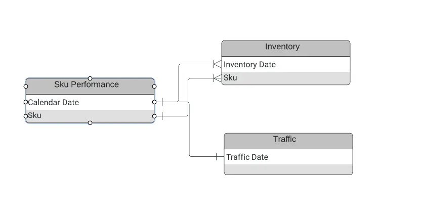
Table construction and notes:

• SKU Performance should be a base table
• LEFT JOIN Inventory on Calendar Date and SKU; LEFT JOIN Traffic on Calendar Date

• Note: You can do this down to the minute depending on the use case. In our examples, inventory will still be joined on the Calendar Date. When going down to the minute, traffic will be joined on the minute instead. 

Relevant Data and Considerations for This Analysis

For this analysis, you’ll need to have access to three sections of your data warehouse: Inventory, Sales, and Website Traffic. 

• Inventory (specifically inventory history) because you’re tracking inventory levels over time
• SKU performance to get through sell-through rate when combined with inventory and to calculate velocity
• Website Traffic as an added data layer on top of sell-through rate determine Inventory / Sales affects during high sales times

You will then be writing/creating additional scripts to generate Inventory History, Sku Performance, and Website Traffic. 

Inventory

Brands often struggle with inventory forecasting because their ERPs do not log historical inventory. Instead, ERPs only provide a snapshot of what you have on hand at a given time. 

For example, if we consider Shopify, via the Inventory API, you can extract inventory_item and inventory_location. 

• Note: In the Shopify API it doesn't provide you the Inventory Date/Time, only the last time the inventory level was changed. This is common across many inventory systems we work with.

So, the first step here is to write a script that will capture your inventory every night, in a table. This way, during a product launch (or any other relevant time, whether during a promotion or other high volume sales period), you can see what your inventory was in a planning/previous period. 

Below is how Daasity handles Inventory history specifically through Shopify.

First, we create a staging table with the most recent inventory snapshot:

INSERT INTO uos_staging.shopify_inventory_levels
SELECT
    il.inventory_item_id AS inventory_level_id
  , il.location_id
  , UPPER(pv.sku) AS sku
  , il.inventory_quantity
  , il.updated_at AS inventory_date
  , CURRENT_TIMESTAMP::TIMESTAMP AS __loaded_at
FROM inventory_levels il
LEFT JOIN locations l ON il.location_id = l.location_id
LEFT JOIN product_variants pv ON il.inventory_item_id = pv.inventory_item_id

We join locations and product variants here from Shopify. We join in locations to account for different locations or types of locations, such as Ecommerce vs. Wholesale or different warehouses. We join to Product Variants since uses an internal ID (inventory_item_id) and it is more readable in the sku format that has been set up. 

From here, we remove inventory levels that are in the staging table. We use this method to retain previous data if that data has been removed from Shopify:

DELETE FROM uos.inventory_levels
WHERE EXISTS
(
  SELECT *
  FROM uos_staging.shopify_inventory_levels il
  WHERE uos.inventory_levels.inventory_level_id = il.inventory_level_id
)

Then, we continue the sync by populating the UOS (our Unified Order Schema) Table. This will get us the most up-to-date inventory level from the inventory snapshot that Shopify provides, at the SKU level:

-- INSERT INTO UOS TABLE
INSERT INTO uos.inventory_levels
SELECT
    inventory_level_id

  , location_id
  , sku
  , inventory_quantity
  , inventory_date
  , __loaded_at
FROM uos_staging.shopify_inventory_levels
;

Finally, we insert the inventory data into a historical table. This provides a leaned down version in the Current Inventory table above while also giving us the ability to look at inventory over time. 

INSERT INTO drp.inventory_level_history
SELECT
	il.inventory_level_id|| ’:’ ||CAST(il.__loaded_at::DATE AS TEXT) AS inventory_history_id
  , il.inventory_level_id
  , il.location_id
  , il.sku
  , il.inventory_quantity
  , il.inventory_date
  , il.__loaded_at
FROM uos.inventory_levels il
WHERE NOT EXISTS
(
  SELECT *
  FROM drp.inventory_level_history ilh
  WHERE ilh.inventory_history_id = il.inventory_level_id|| ‘:’ || CAST(il.__loaded_at::DATE AS TEXT)
)
;

Notes:

1. This inventory sync is based on a daily data refresh; we can calculate what we need for sell-through daily, and it keeps your table structure smaller.
   
   
2. You can use this query for all your inventory systems (Amazon, Netsuite, etc.).
   
   
3. You can expand this analysis to include data from other channels, such as retail or wholesale. Use the “Store Source” field to capture which channel or source you add, or add another column to specify. Some systems will capture from multiple sources, so be sure to account for this change if you add additional inventory sources. 

SKU Performance

The biggest consideration when you’re building your SKU Performance table is to include time when you didn’t sell a product. You need to include active SKUs in any inventory that you may analyze. This can be defined programmatically or through predefined dates. 

Our script runs every night to check updated data to see if the SKU launch date has changed, and it automatically creates a launch date if the launch date has indeed changed. 

However, you don’t want to make this table larger than necessary. For example, you don’t want to create a table that is pulling sales data from the start of time, only when a relevant SKU first launched. 

• E.g., if your company was founded in 2017 and a product wasn’t released until 2022, you can add millions of extra rows by not limiting the date range to post-launch. 
• On the flip side, if a product is discontinued, end the timeframe after the last sale occurred or at the point in time when inventory was depleted

At Daasity, we programmatically determine the launch date. When determining the SKU Launch Date programmatically, there are different scenarios that you need to account for in order to have accurate data.

For example: 

• It’s possible that you may not sell a SKU until a few weeks after launch, for one reason or another
• It’s possible that you may sell SKUs ahead of time, before you acquire inventory. 

For both of these reasons, we look to the first date that either inventory exists or there is a sale of the product. SKU Launch Date:

WITH
  purchase_skus AS
(
  SELECT
  	NVL(oli.shop_id, 'NONE') || ':' || oli.sku AS sku_launch_id
	, oli.shop_id AS store_name
	, oli.sku
	, MIN(o.created_at) AS sku_launch_date
  FROM shopify.order_line_items oli
  LEFT JOIN shopify.orders o ON oli.order_id = o.order_id
  WHERE oli.sku IS NOT NULL
  GROUP BY
  	NVL(oli.shop_id, 'NONE') || ':' || oli.sku AS sku_launch_id
	, oli.shop_id
	, oli.sku
),
  inventory_skus AS
(
  SELECT
  	MD5(NVL(ilh.__shop_id,'NONE') || ':' || ilh.sku) AS sku_launch_id
	, ilh.__shop_id AS store_name
	, ilh.sku
	, MIN(ilh.inventory_date) AS sku_launch_date
  FROM drp.inventory_level_history ilh
  WHERE ilh.sku IS NOT NULL
  GROUP BY
  	MD5(NVL(ilh.__shop_id,'NONE') || ':' || ilh.sku)
	, ilh.__shop_id
	, ilh.sku
),
  all_skus AS
(
  SELECT
  	sku_launch_id
	, store_name
	, sku
	, sku_launch_date
  FROM purchase_skus
  UNION
  SELECT
  	sku_launch_id
	, store_name
	, sku
	, sku_launch_date
  FROM inventory_skus
)
SELECT
	sku_launch_id
  , store_name
  , sku
  , MIN(sku_launch_date) AS sku_launch_date
FROM all_skus
GROUP BY
	sku_launch_id
  , store_name
  , sku

Then, aggregate your sales based on the time period, from the SKU launch date until the present (or desired end date). Within the timeframe, you can adjust the granularity of the sales data depending on your needs. For a general sell-through analysis, breaking it down by day is fine. 

However, for the purposes of this velocity analysis, you probably want your sales data by minute. 

• If your company has been around a while, or if you have a large number of products, we recommend making this a persistent derived table in Looker capitalizing on Liquid Variables for a time period, or limiting the data to specific dates when you run. 

Since the table grows quickly when you go down to the minute, we recommend using Liquid Variables to determine the date (ahead of when you run the query) and passing that through to a PDT. 

We’ve seen that this has been effective in increasing performance while giving the flexibility to examine any date you choose (Note: DATE({% parameter filter_date %}) is the Liquid Variable):

WITH
 row_num AS
(
  SELECT
	ROW_NUMBER() OVER(ORDER BY 1) - 1 AS rn
  FROM shopify.orders
  ORDER BY rn
  LIMIT 1440
),
  sku_performance_date AS
(
  SELECT
	DATEADD(minute, rn.rn , c.calendar_date) AS calendar_date_minute
  FROM drp.calendar c
  CROSS JOIN row_num rn
  WHERE DATE(c.calendar_date) = DATE({% parameter filter_date %})
),
  sku_dates_pre AS
(
SELECT
	MD5(CAST(spd.calendar_date_minute AS TEXT)||':'||sc.store_name||':'||sc.sku) AS sku_performance_id
  , spd.calendar_date_minute
  , sc.sku_launch_date
  , DATEDIFF(day,sc.sku_launch_date,spd.calendar_date_minute) AS days_since_launch
  , sc.store_name
  , sc.sku
FROM drp.sku_launch_date sc
CROSS JOIN sku_performance_date spd
),
  sku_date AS
(
  SELECT
	sku_performance_id
  , calendar_date_minute
  , sku_launch_date
  , days_since_launch
  , store_name
  , sku
  FROM sku_dates_pre
  WHERE days_since_launch >= 0
),
  sku_sales AS
(
  SELECT
  	MD5(CAST(DATE_TRUNC('minute',o.created_at) AS TEXT)||':'||oli.shop_id||':'||oli.sku) AS sku_performance_id
	, DATE_TRUNC('minute',o.created_at) AS order_date_minute
	, oli.shop_id
	, oli.sku
	, SUM(oli.price) AS product_sales_amount
	, SUM(oli.quantity) AS total_quantity
	, SUM(oli.discount_amount) AS discount_amount
  FROM shopify.orders o
  LEFT JOIN shopify.order_line_items oli ON o.order_id = oli.order_id
  WHERE DATE(o.created_at) = DATE({% parameter filter_date %})
  GROUP BY
  	MD5(CAST(DATE_TRUNC('minute',o.created_at) AS TEXT)||':'||oli.shop_id||':'||oli.sku) AS sku_performance_id
	, DATE_TRUNC('minute',o.created_at) AS order_date_minute
	, oli.shop_id
	, oli.sku
)

SELECT
	sd.sku_performance_id
  , sd.calendar_date_minute
  , sd.sku_launch_date
  , sd.days_since_launch
  , sd.store_name
  , sd.sku
  , NVL(ss.product_sales_amount,0) AS product_sales_amount
  , NVL(ss.total_quantity,0) AS total_units
  , NVL(ss.discount_amount, 0) AS discount_amount
FROM sku_date sd
LEFT JOIN sku_sales ss
	ON sd.calendar_date_minute = ss.order_date_minute
	AND sd.store_name = ss.shop_id
	AND sd.sku = ss.sku

Website Traffic

Lastly, you’ll be pulling your site traffic from GA.

If you’re looking to understand aggregate sales velocity without geospecific dimensions, this can be fairly simple, and you can run a query like the one below (you can get the source data from GA through custom reports to get the information down to the minute). 

For our report, we brought in:

• Users
• Sessions
• Page Views
• Transactions
• Product Adds to Cart
• Product Detail Views
• Product List Views
• Quantity Added to Cart
• Date Hour Minute Timestamp

‍

We aggregate by minute using the Liquid Variable to limit this data:

SELECT      	
	CAST((SUBSTRING(date_hour_minute, 1, 4)
	||'-'|| SUBSTRING(date_hour_minute, 5, 2)
  ||'-'|| SUBSTRING(date_hour_minute, 7, 2)
  ||' '|| SUBSTRING(date_hour_minute, 9, 2)
  ||':'|| SUBSTRING(date_hour_minute, 11, 2) || ':00') AS TIMESTAMP) AS date_hour_minute_timestamp    	
	, SUM(users) AS total_users    	
  , SUM(sessions) AS total_sessions    	
  , SUM(page_views) AS total_page_views    	
  , CURRENT_TIMESTAMP::TIMESTAMP AS __loaded_at  	
  
  FROM ga.ga_custom_daily_metrics  	
  WHERE DATE(date_hour_minute_timestamp) = {% parameter filter_date %}
  GROUP BY CAST((SUBSTRING(date_hour_minute, 1, 4)
  ||'-'|| SUBSTRING(date_hour_minute, 5, 2)
  ||'-'|| SUBSTRING(date_hour_minute, 7, 2)
  ||' '|| SUBSTRING(date_hour_minute, 9, 2)
  ||‘:’|| SUBSTRING(date_hour_minute, 11, 2) || ‘:00’) AS TIMESTAMP)

However, if you want to layer in geolocation, your SQL will depend on how you have your UTMs set up (as well as other variables, such as whether you have geospecific Shopify stores). You can add the field “Country ISO Code'' to the custom GA export. 

• You may have minor data inaccuracy, even with UTMs, but this will not significantly affect your data. For example, you may have a customer from France, but they prefer an English website.  

Lastly, please ensure that you verify any custom report(s) from GA. The reports won’t show data if a combination doesn’t exist.So, you will want to verify that when you bring in the fields above,  they match what is expected from GA. 

Adding in Retail Stores

We have also set up this analysis using traffic for retail stores. 

There are tools (e.g., ShopperTrak) that can track traffic that comes in and out of the store. Although they might not be able to determine employees vs. customers, they can give a good idea of how many customers may have visited in a particular time period (e.g., hour, day, week). We followed the same logic above, but only focused on Traffic. 

What you’ll see in Looker

Now that we have assembled the Inventory History, SKU Performance, and Traffic tables, we can combine them into our Explore. 

From there, we can take a look at how effectively we stocked during our sale, how our traffic compared to the sales and sellouts, and more. Here are a few different visualizations we made in Looker that help us answer some of the questions we posed at the beginning of this article. 

Visualization 1: Sessions compared to Sales for a group of SKUs

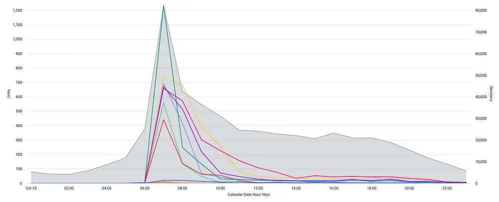
Notice how we run out of inventory early while we still have traffic (from above). In this launch, this answers the question if we stocked better, could we have increased sales for one of these SKUs? 

‍

On the other hand, another SKU was stocked appropriately. 

‍

Visualization 2: Units Sold vs Remaining Inventory (on Hand)

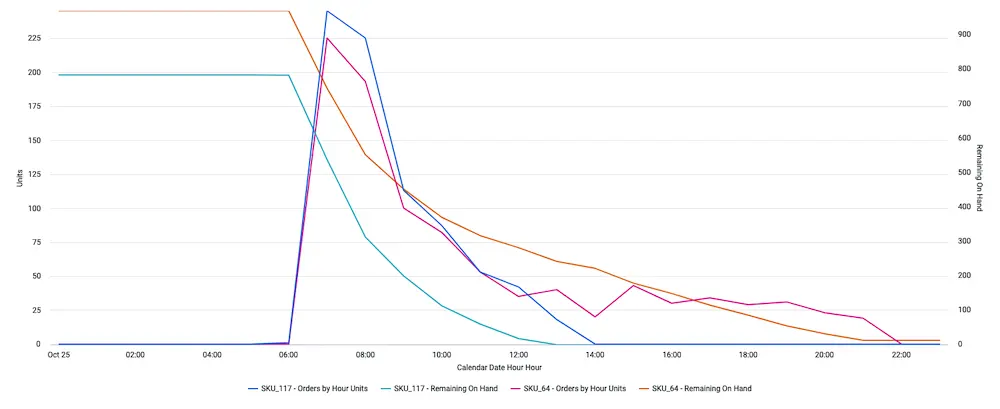
This helps us understand whether stockouts are affecting our site traffic. In this instance, it looks like it. Further, it answers: should we focus on stocking particular items based on a particular {{sku attribute}} such as color, item size, etc. differently? Again, in this instance, yes: an increase in size would be beneficial.

‍

Visualization 3: Total Traffic vs. Sales

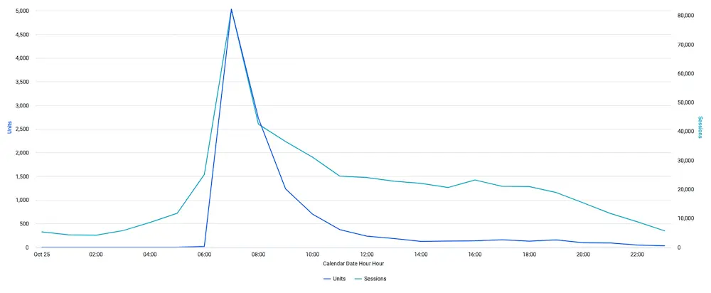
Based on this visualization, it looks like there could still be interest in the sales but that sales really tapered off compared to Traffic. Therefore, an additional marketing push to these sessions, with some additional incentive, could drive them to purchase. 

This answers the question if we are running an all-day sale, would we benefit from a mid-day marketing push on particular products? Answer: yes, a mid-day marketing push would be beneficial to increase sales. 

With further investigation, we can answer which products should we promote?